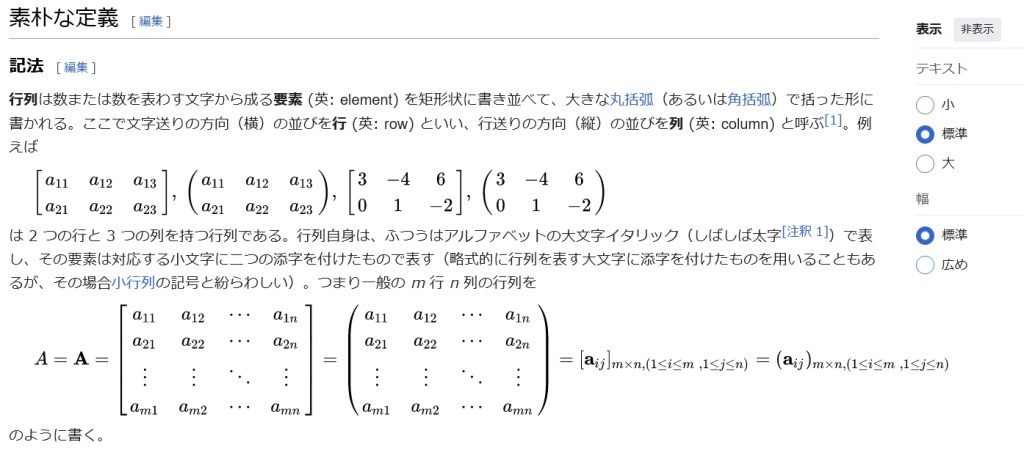
[ a 11 a 12 a 13 a 21 a 22 a 23 ] , ( a 11 a 12 a 13 a 21 a 22 a 23 ) , [ 3 − 4 6 0 1 − 2 ] , ( 3 − 4 6 0 1 − 2 ) {\displaystyle {\begin{bmatrix}a_{11}&a_{12}&a_{13}\\a_{21}&a_{22}&a_{23}\end{bmatrix}},\ {\begin{pmatrix}a_{11}&a_{12}&a_{13}\\a_{21}&a_{22}&a_{23}\end{pmatrix}},\ {\begin{bmatrix}3&-4&6\\0&1&-2\end{bmatrix}},\ {\begin{pmatrix}3&-4&6\\0&1&-2\end{pmatrix}}}
は 2 つの行と 3 つの列を持つ行列である。行列自身は、ふつうはアルファベットの大文字イタリック(しばしば太字[注釈 1])で表し、その要素は対応する小文字に二つの添字を付けたもので表す(略式的に行列を表す大文字に添字を付けたものを用いることもあるが、その場合小行列の記号と紛らわしい)。つまり一般の m 行 n 列の行列を
A = A = [ a 11 a 12 ⋯ a 1 n a 21 a 22 ⋯ a 2 n ⋮ ⋮ ⋱ ⋮ a m 1 a m 2 ⋯ a m n ] = ( a 11 a 12 ⋯ a 1 n a 21 a 22 ⋯ a 2 n ⋮ ⋮ ⋱ ⋮ a m 1 a m 2 ⋯ a m n ) = [ a i j ] m × n , ( 1 ≤ i ≤ m , 1 ≤ j ≤ n ) = ( a i j ) m × n , ( 1 ≤ i ≤ m , 1 ≤ j ≤ n ) {\displaystyle A=\mathbf {A} ={\begin{bmatrix}a_{11}&a_{12}&\cdots &a_{1n}\\a_{21}&a_{22}&\cdots &a_{2n}\\\vdots &\vdots &\ddots &\vdots \\a_{m1}&a_{m2}&\cdots &a_{mn}\end{bmatrix}}={\begin{pmatrix}a_{11}&a_{12}&\cdots &a_{1n}\\a_{21}&a_{22}&\cdots &a_{2n}\\\vdots &\vdots &\ddots &\vdots \\a_{m1}&a_{m2}&\cdots &a_{mn}\end{pmatrix}}=[\mathbf {a} _{ij}]_{m\times n,(1\leq i\leq m\ ,1\leq j\leq n)}=(\mathbf {a} _{ij})_{m\times n,(1\leq i\leq m\ ,1\leq j\leq n)}}
のように書く。
成分
詳細は「行列要素」を参照
書き並べられた要素は行列の成分 (英: entry, component) と呼ばれる[1]。
成分が取り得る値は(さまざまな対象を想定できるが)大抵の場合はある体または可換環 K の元であり、このとき K 上の行列 (英: matrix over K) という。
特に、K が実数全体の成す体 R であるとき実行列と呼び、複素数全体の成す体 C のとき複素行列と呼ぶ。
一つの成分を特定するには、二つの添字が必要である。
行列の第 i 行目、j 列目の成分を特に行列の (i, j) 成分と呼ぶ[1]。
例えば上記行列 A の (1, 2) 成分は a1 2 である。
行列の (i, j) 成分はふつう ai j のように二つの添字を単に横並びに書くが、誤解を避けるために添字の間にコンマを入れることもある。
例えば 1 行 11 列目の成分を a1,11 と書いてよい。
また略式的には、行列 A の (i, j) 成分を指定するのに Ai j という記法を用いることがある。
この場合、例えば積(後述)A B の (i, j) 成分を (A B)i j と指定したりできるので、これで記述の簡素化を図れる場合もある。
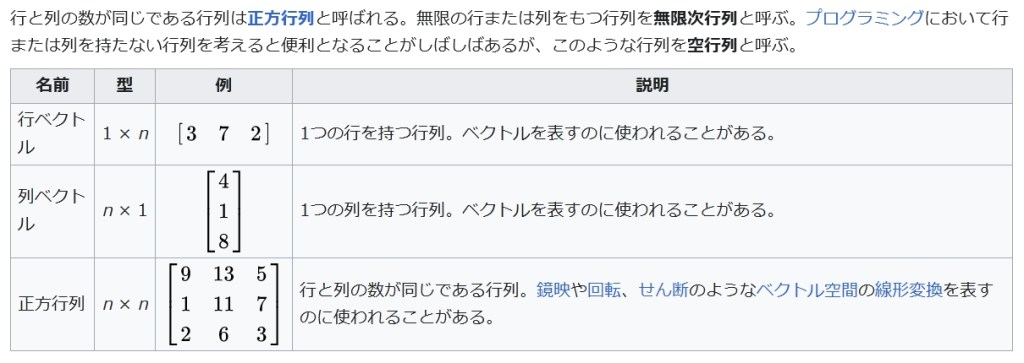
型
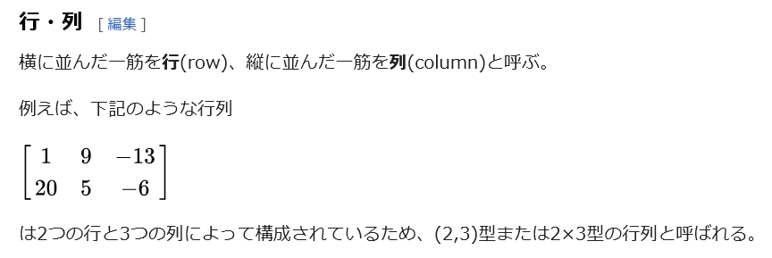
行列に含まれる行の数が m, 列の数が n である時に、その行列を m 行 n 列行列や m × n 行列、m n 行列などと呼ぶ[1]。
行列を構成する行の数と列の数の対を型 (英: type) あるいはサイズという。
したがって m 行 n 列行列のことを (m, n) 型行列などと呼ぶこともある[1]。
K 上の m × n 行列の全体は Km×n, Km,n や Mat(m, n; K), Mm×n(K) などで表される。
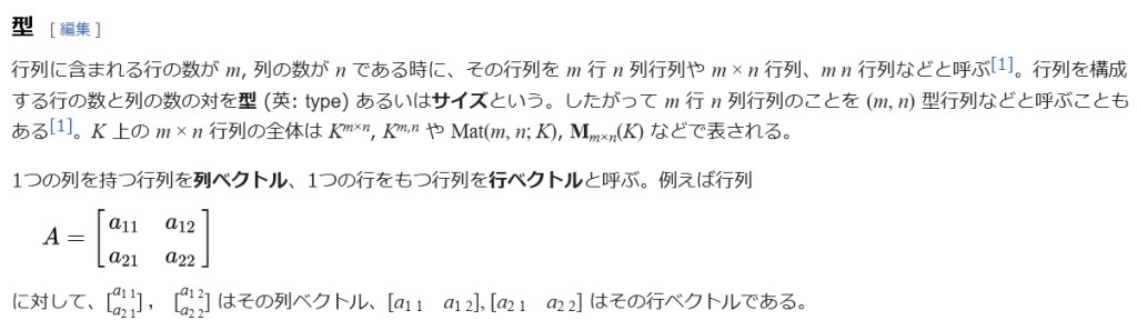
1つの列を持つ行列を列ベクトル、1つの行をもつ行列を行ベクトルと呼ぶ。
例えば行列
A = [ a 11 a 12 a 21 a 22 ] {\displaystyle A={\begin{bmatrix}a_{11}&a_{12}\\a_{21}&a_{22}\end{bmatrix}}}
I have in previous papers defined a "Matrix" as a rectangular array of terms, out of which different systems of determinants may be engendered as from the womb of a common parent. (以前の論文で、項を矩形状に並べた配列として定義した "Matrix" は、そのうちで異なる行列式の体系を生み出す共通の親としての母体である。)
と説明している[8]。
行列式の研究はいくつかの流れから生じてきたものである[9]。
数論的な問題はガウスが二次形式(つまり、 x 2 + x y − 2 y 2 {\displaystyle x^{2}+xy-2y^{2}}のような数式)の係数と三次元の線型写像を行列に結び付けたことに始まり、アイゼンシュタインがこれらの概念をさらに進めて、現代的な用語でいえば行列の積が非可換であることなどを指摘した。
コーシーは行列 A = ( a i j ) {\displaystyle A=(a_{ij})} の行列式として、多項式
a 1 a 2 ⋯ a n ∏ i < j ( a j − a i ) {\displaystyle a_{1}a_{2}\cdots a_{n}\prod _{i<j}(a_{j}-a_{i})}
(ここで ∏ は条件を満たす項の総乗を表す)の冪 a j k を ajk で置き換えたものという定義を採用し、それを用いて行列式についての一般的な主張を証明した最初の人である。
スカラー乗法が意味を持つためには、スカラー λ と行列の成分が同じ環 (K, +, ·, 0) からとった元であるべきであり、このとき m × n 行列の全体 Km×n は、左 K-加群(K が体ならばベクトル空間)になる。ベクトル空間(あるいは自由加群)としての Km×n は m n 次元数ベクトル空間 Km n と同型である。
乗法
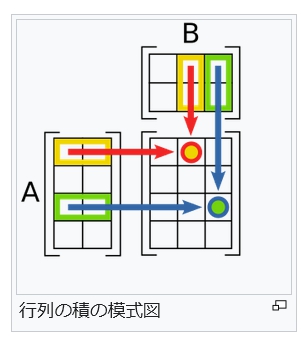
行列の積の模式図
詳細は「行列の乗法」を参照
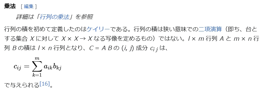
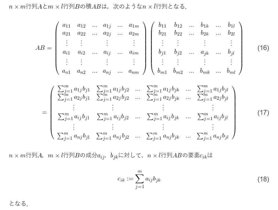
行列の積を初めて定義したのはケイリーである。行列の積は狭い意味での二項演算(即ち、台とする集合 X に対して X × X → X なる写像を定めるもの)ではない。l × m 行列 A と m × n 行列 B の積は l × n 行列となり、C = A B の (i, j) 成分 ci j は、
c i j = ∑ k = 1 m a i k b k j {\displaystyle c_{ij}=\sum _{k=1}^{m}a_{ik}b_{kj}}
即ち一般には
B ⋅ A ≠ A ⋅ B {\displaystyle B\cdot A\neq A\cdot B}
となることが両辺が定義される場合 (l = n) であっても起こり得る。
さらに m = n(= l) のとき、つまり両辺が正方行列同士の積であれば両辺とも定義されるが、その場合でも一般には両者は異なる[16]。
行列の積は結合的である
即ち、乗法が定義される限りにおいて
( A ⋅ B ) ⋅ C = A ⋅ ( B ⋅ C ) {\displaystyle (A\cdot B)\cdot C=A\cdot (B\cdot C)}
が成り立つ[17]。
行列の乗法は加法の上に分配的である
即ち、各項における加法と乗法が定義される限りにおいて
( A + B ) ⋅ C = A ⋅ C + B ⋅ C {\displaystyle (A+B)\cdot C=A\cdot C+B\cdot C}
および
A ⋅ ( B + C ) = A ⋅ B + A ⋅ C {\displaystyle A\cdot (B+C)=A\cdot B+A\cdot C}
が成り立つ[17]。
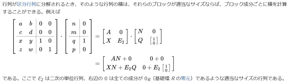
[ a b 0 0 c d 0 0 x y 1 0 z w 0 1 ] ⋅ [ n 0 m 0 q 1 p 0 ] = [ A 0 X E 2 ] ⋅ [ N 0 Q [ 1 0 ] ] = [ A N + 0 0 + 0 X N + E 2 Q 0 + E 2 [ 1 0 ] ] {\displaystyle {\begin{aligned}\left[{\begin{array}{cc|cc}a&b&0&0\\c&d&0&0\\\hline x&y&1&0\\z&w&0&1\end{array}}\right]\cdot \left[{\begin{array}{c|c}n&0\\m&0\\\hline q&1\\p&0\end{array}}\right]&={\begin{bmatrix}A&0\\X&E_{2}\end{bmatrix}}\cdot {\begin{bmatrix}N&0\\Q&\left[{\begin{smallmatrix}1\\0\end{smallmatrix}}\right]\end{bmatrix}}\\&={\begin{bmatrix}AN+0&0+0\\XN+E_{2}Q&0+E_{2}\left[{\begin{smallmatrix}1\\0\end{smallmatrix}}\right]\end{bmatrix}}\end{aligned}}}
である。ここで E2 は二次の単位行列、右辺の 0 は全ての成分が 0R(基礎環 R の零元)であるような適当なサイズの行列である。
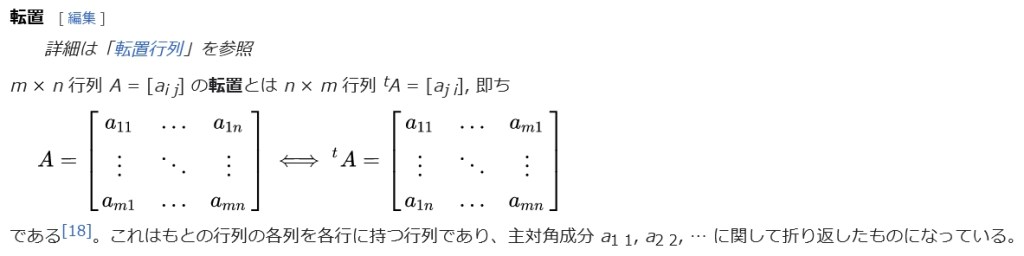
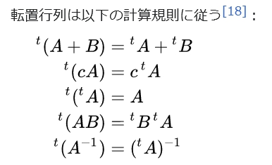
転置
詳細は「転置行列」を参照
m × n 行列 A = [ai j] の転置とは n × m 行列 tA = [aj i], 即ち
A = [ a 11 … a 1 n ⋮ ⋱ ⋮ a m 1 … a m n ] ⟺ t A = [ a 11 … a m 1 ⋮ ⋱ ⋮ a 1 n … a m n ] {\displaystyle A={\begin{bmatrix}a_{11}&\dots &a_{1n}\\\vdots &\ddots &\vdots \\a_{m1}&\dots &a_{mn}\end{bmatrix}}\iff {}^{t}A={\begin{bmatrix}a_{11}&\dots &a_{m1}\\\vdots &\ddots &\vdots \\a_{1n}&\dots &a_{mn}\end{bmatrix}}}
t ( A + B ) = t A + t B t ( c A ) = c t A t ( t A ) = A t ( A B ) = t B t A t ( A − 1 ) = ( t A ) − 1 {\displaystyle {\begin{aligned}{}^{t}(A+B)&={}^{t}A+{}^{t}B\\{}^{t}(cA)&=c\,{}^{t}A\\{}^{t}({}^{t}A)&=A\\{}^{t}(AB)&={}^{t}B\,{}^{t}A\\{}^{t}(A^{-1})&=({}^{t}A)^{-1}\end{aligned}}}
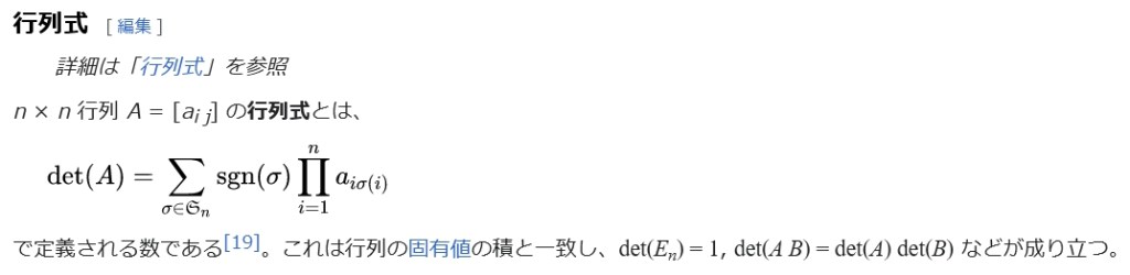
行列式
詳細は「行列式」を参照
n × n 行列 A = [ai j] の行列式とは、
det ( A ) = ∑ σ ∈ S n sgn ( σ ) ∏ i = 1 n a i σ ( i ) {\displaystyle \det(A)=\sum _{\sigma \in {\mathfrak {S}}_{n}}\operatorname {sgn} (\sigma )\prod _{i=1}^{n}a_{i\sigma (i)}}
で定義される数である[19]。
これは行列の固有値の積と一致し、det(En) = 1, det(A B) = det(A) det(B) などが成り立つ。
ランク
詳細は「行列の階数」を参照
行列 A のランクまたは階数とは、この行列の列ベクトルの中で線型独立なものの最大個数であり、また 行ベクトルの中で線型独立なものの最大個数とも等しい[20]。
あるいは A の表現する線型写像の像の次元と言っても同じである[21]。階数・退化次数の定理は、行列の核に階数を加えると、その行列の列の数に等しいことを述べるものである[22]。 トレース 詳細は「跡 (線型代数学)」を参照
n × n 行列 A = [ai j] のトレースまたは跡とは、その対角線上にある成分の和
tr ( A ) = a 11 + a 22 + ⋯ + a n n {\displaystyle \operatorname {tr} (A)=a_{11}+a_{22}+\dotsb +a_{nn}}
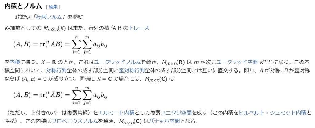
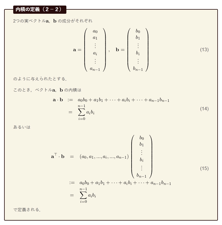
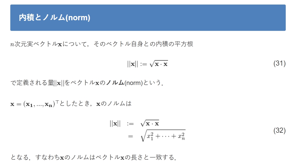
のことである[23]。これは tr(A B) = tr(B A) を満たし[23]、行列のトレースはその固有値の和に等しい。 内積とノルム 詳細は「行列ノルム」を参照
K-加群としての Mm×n(K) はまた、行列の積 tA B のトレース
⟨ A , B ⟩ = tr ( t A B ) = ∑ i = 1 n ∑ j = 1 m a i j b i j {\displaystyle \langle A,B\rangle =\operatorname {tr} ({}^{t}AB)=\sum _{i=1}^{n}\sum _{j=1}^{m}a_{ij}b_{ij}}
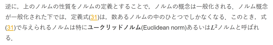
を内積に持つ。K = R のとき、これはユークリッドノルムを導き、Mm×n(R) は m n-次元ユークリッド空間 Km n になる。この内積空間において、対称行列全体の成す部分空間と歪対称行列全体の成す部分空間とは互いに直交する。即ち、A が対称, B が歪対称ならば ⟨A, B⟩ = 0 が成り立つ。同様に K = C の場合には、Mm×n(C) は
⟨ A , B ⟩ = tr ( t A ¯ B ) = ∑ i = 1 n ∑ j = 1 m a ¯ i j b i j {\displaystyle \langle A,B\rangle =\operatorname {tr} ({}^{t}{\bar {A}}B)=\sum _{i=1}^{n}\sum _{j=1}^{m}{\bar {a}}_{ij}b_{ij}}
任意の行列 B に対し、その成分をそれぞれの成分の加法逆元に全て取り換えた行列を −B と書けば、同じサイズの行列 A, B の和 A + (−B) を A − B と略記して差を定めることができる[注釈 3]。より強く、スカラー乗法が定義される場合には、特にスカラー (−1)-倍は (−1)B = −B を満たすのだから、和とスカラー倍を使って差を定義することもできる。
n × n の正方行列 A に対して行列のべき乗は An (ここで n は実数) と書かれる[24]。
行列 A が対角化可能であれば、An = (P−1DP)n = P−1DnP として容易に計算できる。 ベクトルの二項積
v と w を n × 1 の列ベクトルとすると、v と w との間に行列の積は定義されないが、tv w および v tw は行列の積として定義することができる。前者は 1 × 1 行列であり、これをスカラーと解釈すれば、v と w との標準内積 ⟨v, w⟩ に他ならない。いっぽう後者は、階数 1 の n × n 行列で、v と w との二項積 v w あるいはテンソル積 v ⊗ w と呼ばれる。 行列の三項積
可換環 K 上の m × n 行列の全体 Mm×n(K) は加法とスカラー倍について K-加群を成すばかりでなく、その上の三項演算
M m × n ( K ) × M m × n ( K ) × M m × n ( K ) → M m × n ( K ) ; ( X , Y , Z ) ↦ { X , Y , Z } := X t Y Z {\displaystyle M_{m\times n}(K)\times M_{m\times n}(K)\times M_{m\times n}(K)\to M_{m\times n}(K);\quad (X,Y,Z)\mapsto \{X,Y,Z\}:=X\,{}^{t}Y\,Z}
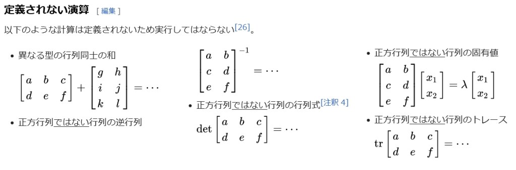
異なる型の行列同士の和
[ a b c d e f ] + [ g h i j k l ] = ⋯ {\displaystyle {\begin{bmatrix}a&b&c\\d&e&f\end{bmatrix}}+{\begin{bmatrix}g&h\\i&j\\k&l\end{bmatrix}}=\cdots }
正方行列ではない行列の逆行列
[ a b c d e f ] − 1 = ⋯ {\displaystyle {\begin{bmatrix}a&b\\c&d\\e&f\end{bmatrix}}^{-1}=\cdots }
正方行列ではない行列の行列式[注釈 4]
det [ a b c d e f ] = ⋯ {\displaystyle \det {\begin{bmatrix}a&b&c\\d&e&f\end{bmatrix}}=\cdots }
正方行列ではない行列の固有値
[ a b c d e f ] [ x 1 x 2 ] = λ [ x 1 x 2 ] {\displaystyle {\begin{aligned}{\begin{bmatrix}a&b\\c&d\\e&f\end{bmatrix}}{\begin{bmatrix}x_{1}\\x_{2}\end{bmatrix}}=\lambda \,{\begin{bmatrix}x_{1}\\x_{2}\end{bmatrix}}\\\end{aligned}}}
正方行列ではない行列のトレース
tr [ a b c d e f ] = ⋯ {\displaystyle \operatorname {tr} {\begin{bmatrix}a&b&c\\d&e&f\end{bmatrix}}=\cdots }
行列の分解 詳細は「行列の分解」を参照
行列を2つあるいは3つの行列の積に因数分解するには以下の方法が知られている。
LU分解 - 正方行列Aを下三角行列と上三角行列の積に分解。 A = LU
コレスキー分解 - 正値対称行列(またはエルミート行列)Aを下三角行列と上三角行列の積に分解。 A = U*U
QR分解 - (m,n)行列を直交行列(またはユニタリ行列)Qと上三角行列Rに分解 A = QR
固有値分解 -
特異値分解 - (m,n)行列を直交行列(またはユニタリ行列)U,Vと対角行列Dに分解 A = UDV*
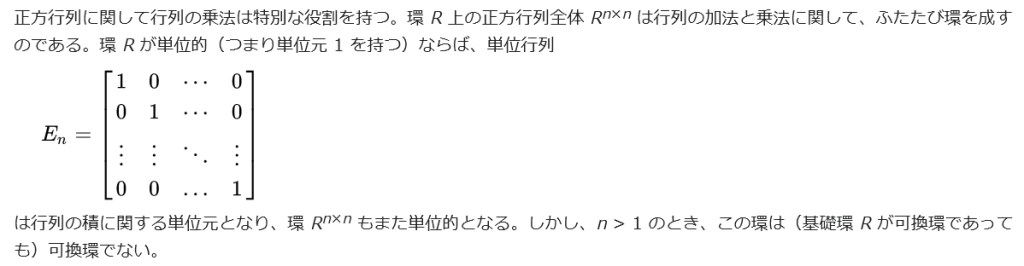
しばしば実または複素成分の行列に焦点を当てることもあるが、それ以外にももっと一般の種類の成分を持った行列を考えることができる。一般化の最初の段階として任意の体(すなわち四則演算が自由にできる集合、例えば R, C 以外に有理数体 Q や有限体 Fqなど)を成分として考える。例えば符号理論では有限体上の行列を利用する。どの体で考えるとしても、固有値は多項式の根として考えることができて、それは行列の係数体の拡大体の中に存在する。たとえば、実行列の場合は固有値は複素数である。ある行列の成分をより大きな体の元と解釈しなおすことはできる(例えば実行列を全ての成分が実数であるような複素行列とみることができる)から、そのような十分大きな体の中で任意の正方行列についてその固有値全てから成る集合を考えることができる。あるいは最初から、複素数体 C のような代数閉体に成分を持つような行列のみを考えるものとすることもできる。
もっと一般に、抽象代数学では環に成分を持つ行列というものが甚だ有用である[30]。環は除法演算を持たない点において体よりも一般の概念である。この場合も、行列の加法と乗法はそのまままったく同じ物を使うことができる。R 上の n-次正方行列全体の成す集合 M(n, R) は全行列環と呼ばれる環であり、左 R-加群 Rn の自己準同型環に同型である[31]。環 R が可換環、すなわちその乗法が可換律を満たすならば、全行列環 M(n, R) は(n = 1 でない限り)非可換な R 上の単位的結合多元環となる。可換環 R 上の正方行列の行列式はライプニッツの公式を用いて定義することができて、可換環 R 上の正方行列が可逆であることの必要十分条件をその行列式が R の可逆元であることと述べることができる(これは零元でない任意の元が可逆元であった体の場合の一般化になっている)[32]。超環(英語版)上の行列は超行列(英語版)と呼ばれる[33]。
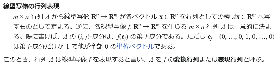
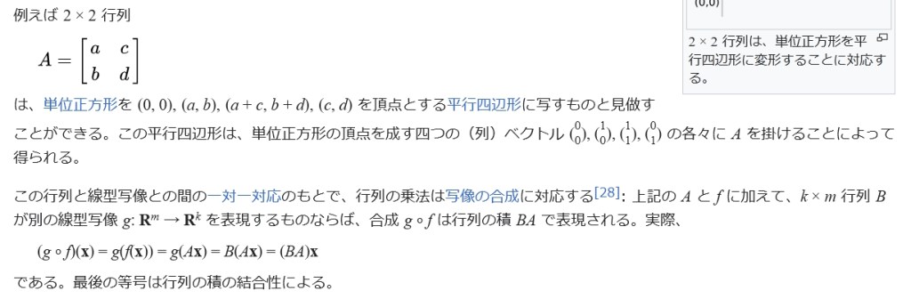
線型写像 Rn → Rm は既に述べたように m × n 行列と等価である。一般に有限次元ベクトル空間の間の線型写像 f: V → W は(V の次元を n, W の次元を m として) V の基底 v1, …, vn と W の基底 w1, …, wm を選べば
f ( v j ) = ∑ i = 1 m a i , j w i ( j = 1 , … , n ) {\displaystyle f(\mathbf {v} _{j})=\sum _{i=1}^{m}a_{i,j}\mathbf {w} _{i}\quad (j=1,\ldots ,n)}
を満たす行列 A = (aij) によって記述することができる。言い換えれば、 A の第 j-列は基底ベクトル vj の像を W の基底 {wi} に関して表したものになっている。従ってこのような関係は行列 A の成分から一意的に定まる。注意すべきは線型写像を表す行列は基底の取り方に依存することである。基底の取り方を変えれば別な行列が生じるが、それはもとの行列と同値になる[34]。既に述べた具体的な概念の多くはこの方法を通して解釈しなおすことができる。例えば転置行列 A⊤ は A の定める線型写像の転置写像を、双対基底に関して記述するものである。[35]。
より一般に、m × n 行列全体の成す集合は、勝手な単位的環 R に対して自由加群 Rm および Rn の間の R-線型写像を表すのに利用することができる。n = m のとき、そのような写像の合成を定義することができて、n-次正方行列全体の成す全行列環が、Rn の自己準同型環を表現するものとして生じる。 行列群 詳細は「線型代数群」を参照
R を任意の単位的環とすれば、右 R-加群としての M = ⨁ i ∈ I R {\displaystyle \textstyle M=\bigoplus _{i\in I}R} の自己準同型環は、I × I で添字付けられ、各列の非零成分の数が有限個であるような列有限行列の環 CFMI(R) に同型である。これと対応するものとして、左 R-加群としての M の自己準同型環を考えれば、同様に各行の非零成分の数が有限な行有限行列の環 RFMI(R) が得られる。
無限次元行列を線型写像を記述するのに用いるならば、次に述べるような理由から、その各列ベクトルが有限個の例外を除いて全ての成分が 0 となるものとならなければ無用である。A が適当な基底に関して線型写像 f: V → W を表現するものとすると、それは定義により、空間の任意のベクトルを基底ベクトルの(有限)線型結合として一意に表すことによって与えられるのであるから、従って(列)ベクトル v の成分 vi で非零となるものは有限個に限られる。また、A の各列は V の各基底ベクトルの f による像を W の基底に関して表したものとなっているから、これが意味を持つのはこれらの列ベクトルの非零成分が有限個である場合に限る。しかし一方で、A の行に関しては何の制約もない。事実、v の非零成分が有限個であるならば、積 Av はその各成分が見かけ上無限和の形で与えられるとしても、実際にはそれは非零の項が有限個しかないから、間違いなく決定することができる。さらに言えば、これは A の実質的に有限個の列の線型結合を成すことになり、また各列の非零成分は有限個だから結果として得られる和も非零成分が有限個になる。(通常は、行と列が同じ集合で添字付けられるような)与えられた型の二つの行列の積は矛盾無く定義できて、もとと同じ型を持ち、線型写像の合成に対応することも確認できる。
R がノルム環ならば、行または列に関する有限性条件を緩めることができる。すなわち、有限和の代わりに、そのノルムに関する絶対収束級数を考えればよい。例えば、列和が絶対収束列となるような行列の全体は環を成す。もちろん同様に、行和が絶対収束列となるような行列の全体も環を成す。
^ 下線や二重下線などを付けることもあるが、これはタイプライター原稿で用いられた太字書体を指示する書式の名残[2]
^ OEDによれば、数学用語としての "matrix" の最初の用例は J. J. Sylvester in London, Edinb. & Dublin Philos. Mag. 37 (1850), p. 369: "We ‥commence‥ with an oblong arrangement of terms consisting, suppose, of m lines and n columns. This will not in itself represent a determinant, but is, as it were, a Matrix out of which we may form various systems of determinants by fixing upon a number p, and selecting at will p lines and p columns, the squares corresponding to which may be termed determinants of the pth order.
^ これは与えられた行列の全ての成分が加法逆元を持つ限りにおいて、加法のみから定められることに注意。特にスカラー乗法が(任意のスカラーと任意の行列に対する演算として)定義されている必要はない。従って、同じサイズの任意の行列に対する減法を定めるならば、例えば係数域が加法についてアーベル群であれば十分であるが、通例として行列の係数域は何らかの可換環と仮定するから、それには環の加法群構造を用いればよい
^ 正方行列でない行列に対して行列式を考える理論も存在する。これは C. E. Cullis により導入された。[27]
^ 普通はさらに一般線型群の閉集合となることも要求する。
^ "Not much of matrix theory carries over to infinite-dimensional spaces, and what does is not so useful, but it sometimes helps." [42]
^ "Empty Matrix: A matrix is empty if either its row or column dimension is zero",[43] "A matrix having at least one dimension equal to zero is called an empty matrix", [44]
出典
^ a b c d e 斎藤2017、21頁。
^ https://raksul.com/dictionary/underline/
^ Shen, Crossley & Lun 1999 cited by Bretscher 2005, p. 1
^ Needham, Joseph; Wang Ling (1959). Science and Civilisation in China. III. Cambridge: Cambridge University Press. p. 117. ISBN 9780521058018
^ Cayley 1889, pp. 475–496, vol. II.
^ Dieudonné 1978, p. 96, Vol. 1, Ch. III.
^ Merriam–Webster dictionary, Merriam–Webster 2009年4月20日閲覧。
^ The Collected Mathematical Papers of James Joseph Sylvester: 1837–1853, Paper 37, p. 247
^ Knobloch 1994.
^ Hawkins 1975.
^ Kronecker 1897.
^ Weierstrass 1915, pp. 271–286.
^ Bôcher 2004.
^ Mehra & Rechenberg 1987.
^ a b c d 斎藤2017、23頁。
^ a b 斎藤2017、24頁。
^ a b 斎藤2017、25頁。
^ a b 斎藤2017、31頁。
^ 斎藤2017、89頁。
^ Brown 1991, Definition II.3.3.
^ Greub 1975, Section III.1.
^ Brown 1991, Theorem II.3.22.
^ a b 斎藤2017、34頁。
^ 斎藤2017、26頁。
^ http://www2.math.kyushu-u.ac.jp/~tnomura/EdAct/2010TKR.pdf
^ Stephen P. Boyd. “Crimes against Matrices” (pdf). 2013年3月2日閲覧。
^ 中神祥臣・柳井晴夫 著、『矩形行列の行列式』、丸善、2012年。ISBN 978-4-621-06508-2.
^ Greub 1975, Section III.2.
^ Coburn 1955, Ch. V.
^ Lang 2002, Chapter XIII.
^ Lang 2002, XVII.1, p. 643.
^ Lang 2002, Proposition XIII.4.16.
^ Reichl 2004, Section L.2.
^ Greub 1975, Section III.3.
^ Greub 1975, Section III.3.13.
^ Baker 2003, Def. 1.30.
^ Baker 2003, Theorem 1.2.
^ Artin 1991, Chapter 4.5.
^ Artin 1991, Theorem 4.5.13.
^ Rowen 2008, Example 19.2, p. 198.
^ Itõ 1987, "Matrix".
^ Halmos 1982, p. 23, Chapter 5.
^ Glossary, O-Matrix v6 User Guide.
^ MATLAB Data Structures
参考文献
Arnold, V. I.; Cooke, Roger (1992), Ordinary differential equations, Berlin, New York: Springer-Verlag, ISBN 978-3-540-54813-3
Artin, Michael (1991), Algebra, Prentice Hall, ISBN 978-0-89871-510-1
Association for Computing Machinery (1979), Computer Graphics, Tata McGraw–Hill, ISBN 978-0-07-059376-3
Baker, Andrew J. (2003), Matrix Groups: An Introduction to Lie Group Theory, Berlin, New York: Springer-Verlag, ISBN 978-1-85233-470-3
Bau III, David; Trefethen, Lloyd N. (1997), Numerical linear algebra, Philadelphia: Society for Industrial and Applied Mathematics, ISBN 978-0-89871-361-9
Bretscher, Otto (2005), Linear Algebra with Applications (3rd ed.), Prentice Hall
Bronson, Richard (1989), Schaum's outline of theory and problems of matrix operations, New York: McGraw–Hill, ISBN 978-0-07-007978-6
Brown, William A. (1991), Matrices and vector spaces, New York: M. Dekker, ISBN 978-0-8247-8419-5
Coburn, Nathaniel (1955), Vector and tensor analysis, New York: Macmillan, OCLC 1029828
Conrey, J. B. (2007), Ranks of elliptic curves and random matrix theory, Cambridge University Press, ISBN 978-0-521-69964-8
Fudenberg, D.; Tirole, Jean (1983), Game Theory, MIT Press
Gilbarg, David; Trudinger, Neil S. (2001), Elliptic partial differential equations of second order (2nd ed.), Berlin, New York: Springer-Verlag, ISBN 978-3-540-41160-4
Godsil, Chris; Royle, Gordon (2004), Algebraic Graph Theory, Graduate Texts in Mathematics, 207, Berlin, New York: Springer-Verlag, ISBN 978-0-387-95220-8
Golub, Gene H.; Van Loan, Charles F. (1996), Matrix Computations (3rd ed.), Johns Hopkins, ISBN 978-0-8018-5414-9
Golub, Gene H.; Van Loan, Charles F. (2013), Matrix Computations (4th ed.), Johns Hopkins, ISBN 978-1-4214-0794-4
Greub, Werner Hildbert (1975), Linear algebra, Graduate Texts in Mathematics, Berlin, New York: Springer-Verlag, ISBN 978-0-387-90110-7
Halmos, Paul Richard (1982), A Hilbert space problem book, Graduate Texts in Mathematics, 19 (2nd ed.), Berlin, New York: Springer-Verlag, ISBN 978-0-387-90685-0, MR675952
Horn, Roger A.; Johnson, Charles R. (2013). Matrix analysis (Second ed.). Cambridge University Press. ISBN 978-0-521-54823-6. MR2978290
Householder, Alston S. (1975), The theory of matrices in numerical analysis, New York: Dover Publications, MR0378371
Krzanowski, W. J. (1988), Principles of multivariate analysis, Oxford Statistical Science Series, 3, The Clarendon Press Oxford University Press, ISBN 978-0-19-852211-9, MR969370
Itõ, Kiyosi, ed. (1987), Encyclopedic dictionary of mathematics. Vol. I--IV (2nd ed.), MIT Press, ISBN 978-0-262-09026-1, MR901762
Lang, Serge (1969), Analysis II, Addison-Wesley
Lang, Serge (1987a), Calculus of several variables (3rd ed.), Berlin, New York: Springer-Verlag, ISBN 978-0-387-96405-8
Lang, Serge (1987b), Linear algebra, Berlin, New York: Springer-Verlag, ISBN 978-0-387-96412-6
Lang, Serge (2002), Algebra, Graduate Texts in Mathematics, 211 (Revised third ed.), New York: Springer-Verlag, ISBN 978-0-387-95385-4, MR1878556
Latouche, G.; Ramaswami, V. (1999), Introduction to matrix analytic methods in stochastic modeling (1st ed.), Philadelphia: Society for Industrial and Applied Mathematics, ISBN 978-0-89871-425-8
Manning, Christopher D.; Schütze, Hinrich (1999), Foundations of statistical natural language processing, MIT Press, ISBN 978-0-262-13360-9
Mehata, K. M.; Srinivasan, S. K. (1978), Stochastic processes, New York: McGraw–Hill, ISBN 978-0-07-096612-3
Mirsky, Leonid (1990), An Introduction to Linear Algebra, Courier Dover Publications, ISBN 978-0-486-66434-7
Nocedal, Jorge; Wright, Stephen J. (2006), Numerical Optimization (2nd ed.), Berlin, New York: Springer-Verlag, p. 449, ISBN 978-0-387-30303-1
Oualline, Steve (2003), Practical C++ programming, O'Reilly, ISBN 978-0-596-00419-4
Press, William H.; Flannery, Brian P.; Teukolsky, Saul A.; Vetterling, William T. (1992), “LU Decomposition and Its Applications”, Numerical Recipes in FORTRAN: The Art of Scientific Computing (2nd ed.), Cambridge University Press, pp. 34–42
Punnen, Abraham P.; Gutin, Gregory (2002), The traveling salesman problem and its variations, Boston: Kluwer Academic Publishers, ISBN 978-1-4020-0664-7
Reichl, Linda E. (2004), The transition to chaos: conservative classical systems and quantum manifestations, Berlin, New York: Springer-Verlag, ISBN 978-0-387-98788-0
Rowen, Louis Halle (2008), Graduate Algebra: noncommutative view, Providence, R.I.: American Mathematical Society, ISBN 978-0-8218-4153-2
Šolin, Pavel (2005), Partial Differential Equations and the Finite Element Method, Wiley-Interscience, ISBN 978-0-471-76409-0
Stinson, Douglas R. (2005), Cryptography, Discrete Mathematics and Its Applications, Chapman & Hall/CRC, ISBN 978-1-58488-508-5
Stoer, Josef; Bulirsch, Roland (2002), Introduction to Numerical Analysis (3rd ed.), Berlin, New York: Springer-Verlag, ISBN 978-0-387-95452-3
Ward, J. P. (1997), Quaternions and Cayley numbers, Mathematics and its Applications, 403, Dordrecht: Kluwer Academic Publishers Group, ISBN 978-0-7923-4513-8, MR1458894
Wolfram, Stephen (2003), The Mathematica Book (5th ed.), Champaign, Ill: Wolfram Media, ISBN 978-1-57955-022-6
Pappur Nagappa Shivakumar、K C Sivakumar、Yang Zhang: "Infinite Matrices and Their Recent Applications", Springer, ISBN 978-3319301792 (2016年5月25日)。
斎藤正彦『線形代数学』(第3版)東京図書、2017年4月10日。ISBN 978-4-489-02179-4。
物理学に関するもの
Bohm, Arno (2001), Quantum Mechanics: Foundations and Applications, Springer, ISBN 0-387-95330-2
Burgess, Cliff; Moore, Guy (2007), The Standard Model. A Primer, Cambridge University Press, ISBN 0-521-86036-9
Guenther, Robert D. (1990), Modern Optics, John Wiley, ISBN 0-471-60538-7
Itzykson, Claude; Zuber, Jean-Bernard (1980), Quantum Field Theory, McGraw–Hill, ISBN 0-07-032071-3
Riley, K. F.; Hobson, M. P.; Bence, S. J. (1997), Mathematical methods for physics and engineering, Cambridge University Press, ISBN 0-521-55506-X
Schiff, Leonard I. (1968), Quantum Mechanics (3rd ed.), McGraw–Hill
Weinberg, Steven (1995), The Quantum Theory of Fields. Volume I: Foundations, Cambridge University Press, ISBN 0-521-55001-7
Wherrett, Brian S. (1987), Group Theory for Atoms, Molecules and Solids, Prentice–Hall International, ISBN 0-13-365461-3
Zabrodin, Anton; Brezin, Édouard; Kazakov, Vladimir; Serban, Didina; Wiegmann, Paul (2006), Applications of Random Matrices in Physics (NATO Science Series II: Mathematics, Physics and Chemistry), Berlin, New York: Springer-Verlag, ISBN 978-1-4020-4530-1
歴史に関するもの
Bôcher, Maxime (2004), Introduction to higher algebra, New York: Dover Publications, ISBN 978-0-486-49570-5, reprint of the 1907 original edition
Cayley, Arthur (1889), The collected mathematical papers of Arthur Cayley, I (1841–1853), Cambridge University Press, pp. 123–126
Dieudonné, Jean, ed. (1978), Abrégé d'histoire des mathématiques 1700-1900, Paris: Hermann
Hawkins, Thomas (1975), “Cauchy and the spectral theory of matrices”, Historia Mathematica 2: 1–29, doi:10.1016/0315-0860(75)90032-4, ISSN 0315-0860, MR0469635
Knobloch, Eberhard (1994), “From Gauss to Weierstrass: determinant theory and its historical evaluations”, The intersection of history and mathematics, Sci. Networks Hist. Stud., 15, Basel, Boston, Berlin: Birkhäuser, pp. 51–66, MR1308079
Kronecker, Leopold (1897), Hensel, Kurt, ed., Leopold Kronecker's Werke, Teubner
Mehra, J.; Rechenberg, Helmut (1987), The Historical Development of Quantum Theory (1st ed.), Berlin, New York: Springer-Verlag, ISBN 978-0-387-96284-9
Shen, Kangshen; Crossley, John N.; Lun, Anthony Wah-Cheung (1999), Nine Chapters of the Mathematical Art, Companion and Commentary (2nd ed.), Oxford University Press, ISBN 978-0-19-853936-0
Weierstrass, Karl (1915), Collected works, 3
Online Matrix Multiplication using AJAX
Online Inverse Matrix Calculator using AJAX
Online Calculator - Operation with matrices in R (determinant, track, inverse, adjoint, transpose)
『行列』 - コトバンク
歴史
MacTutor: Matrices and determinants
Matrices and Linear Algebra on the Earliest Uses Pages
Earliest Uses of Symbols for Matrices and Vectors
オンライン本
Kaw, Autar K., Introduction to Matrix Algebra, ISBN 978-0-615-25126-4
The Matrix Cookbook 2008年12月10日閲覧。
Brookes, M. (2005), The Matrix Reference Manual, London: Imperial College 2008年12月10日閲覧。
『行列および行列式』荒又秀夫著、東海書房、1947年刊
オンラインの行列計算器
SuperiorMath (Matrix Calculator)
Matrix Calculator (DotNumerics )
Xiao, Gang, Matrix calculator 2008年12月10日閲覧。
Online matrix calculator 2008年12月10日閲覧。
Online matrix calculator(ZK framework) 2009年11月26日閲覧。
Oehlert, Gary W.; Bingham, Christopher, MacAnova, University of Minnesota, School of Statistics 2008年12月10日閲覧。, a freeware package for matrix algebra and statistics
Online matrix calculator 2009年12月14日閲覧。
Operation with matrices in R (determinant, track, inverse, adjoint, transpose)
Matrix Formulas
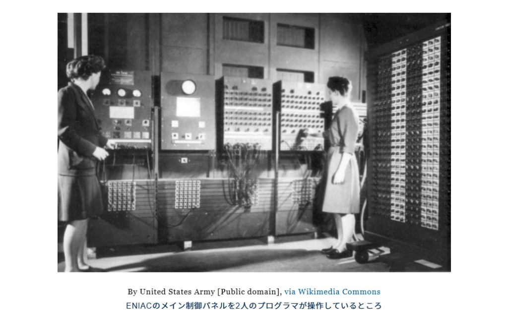
フォン・ノイマンは、チューリングのチューリングマシンの論文を読み、チューリングマシンでは、プログラムをデータと同じように扱っていたことに衝撃を受けます。フォン・ノイマンは、この発想を応用すれば、「ケーブル接続された巨大電卓」を「電子頭脳」に進化させることができると気がつきます。 two women operating the ENIAC’s main control panel
By United States Army [Public domain], via Wikimedia Commons ENIACのメイン制御パネルを2人のプログラマが操作しているところ プログラムとデータを同列で扱うフォン・ノイマン型コンピューター
チューリングマシン M は次の7つ組で定義される:

M = ? Q , Γ , b , Σ , δ , q i n i t , q a c c ? . {\displaystyle M=\langle Q,{\mathit {\Gamma }},b,{\mathit {\Sigma }},\delta ,q_{\mathrm {init} },q_{\mathrm {acc} }\rangle \,.}
状態 有限集合 Q の元 q ∈ Q を状態 (state) という。
字母・記号・文字列 状態集合 Q と交わらない有限集合 Γ を字母(alphabet)といい、字母の元 a ∈ Γ を記号 (symbol) という。重複を許した有限個の記号の列全体からなる集合を Γ* と表し、その元 x ∈ Γ* を字母 Γ の文字列(string)または文(statement)という。
遷移函数 写像 δ: Q × Γ → Q × Γ × {left, right} を遷移函数という。δ(q, a) = (q′, a′, m) は、「現在の状態が q であり、着目位置の記号が a であれば、状態を q′ に移し、着目位置に記号 a′ を書き込んでから、着目位置を m ∈ {left, right} 方向に1つずらす」と読む。
初期状態 状態集合 Q のある元 qinit を初期状態(initial state)と定める。
受理状態 状態集合 Q のある元 qacc を受理状態(accepting state)と定める。
状況 Γ ∪ Q {\textstyle {\mathit {\Gamma }}\cup Q} 上の(片側)無限列のうち、状態集合 Q の元がちょうど1度現れ、また空白 b 以外の記号が有限回しか現れないものをチューリングマシン M の状況(configuration)という。遷移函数 δ は、状況から状況への写像を自然に定める。
受理 「チューリングマシン M が入力文字列 x ∈ Σ ? {\textstyle x\in \Sigma ^{*}} を受理(accept)する」とは、チューリングマシン M が初期状態 qinit で入力文字列 x が与えられた状況 q i n i t x b b ? {\textstyle q_{\mathrm {init} }xbb\cdots } に対し、遷移函数 δ を有限回作用させ受理状態 qacc へ遷移した状況 q a c c b b ? {\textstyle q_{\mathrm {acc} }bb\cdots } が得られることをいう。
実行時間・記憶領域量 チューリングマシン M が入力文字列 x ∈ Σ* を受理するまで遷移函数を作用させる最小の回数をチューリングマシン M の入力文字列 x に対する実行時間とよぶ。その過程における状況中の q の最右位置を、M が x に対して使用する記憶領域量という。
M が言語 L ⊆ Σ ? {\displaystyle L\subseteq {\mathit {\Sigma }}^{}} を認識するとは、M が L の元のみをみな受理することをいう。そのようなチューリング機械 M が存在するとき、L は帰納可枚挙(recursively enumerable)あるいは計算可枚挙(computably enumerable)であるという。L と Σ ? ? L {\displaystyle {\mathit {\Sigma }}^{}\setminus L} がともに帰納可枚挙であるとき、Lは帰納的(recursive)あるいは決定可能(decidable)であるという。
より精細に、自然数から自然数への写像 t に対し、M が L を時間計算量[ないし空間計算量]t で認識するとは、M が L を認識し、かつ各 x ∈ L {\displaystyle x\in L} に対する M {\displaystyle M} の実行時間[ないし記憶領域量]が t ( | x | ) {\displaystyle t(\left|x\right|)} 以下であることをいう。ここで | x | {\displaystyle \left|x\right|} は文字列 x の長さを表す。
すなわち、遷移函数 δ {\displaystyle \delta }を Q × Γ 2 {\displaystyle Q\times {\mathit {\Gamma }}^{2}}から Q × Γ × { l e f t , r i g h t } 2 {\displaystyle Q\times {\mathit {\Gamma }}\times {\mathrm {left} ,\mathrm {right} }^{2}}への写像とし、状況の定義も適切に変更する。
すなわち機械 M {\displaystyle M}は、各 x ∈ d o m ( f ) {\displaystyle x\in \mathrm {dom} (f)}に対しては文字列 f ( x ) {\displaystyle f(x)}をテープに書いてから初めて受理状態へ移り、 x ? d o m ( f ) {\displaystyle x\notin \mathrm {dom} (f)}に対しては決して受理状態へ移らない。このような M {\displaystyle M}が存在するとき、 f {\displaystyle f}は部分帰納的あるいは計算可能(computable)であるという。
決定的と非決定的
遷移関数 δ {\displaystyle \delta }において、現在の状態 q と着目位置にある記号 a の、ある組 (q, a) に対し、値(すなわちその時にすべき動作)が、高々一つならば、そのチューリングマシンは「決定的」(deterministic)である。
^ "チューリングマシン". ASCII.jpデジタル用語辞典. コトバンクより2022年2月2日閲覧。
^ Turing, A. M. (1937). “On Computable Numbers, with an Application to the Entscheidungsproblem” (英語). Proceedings of the London Mathematical Society s2-42 (1): 230?265. doi:10.1112/plms/s2-42.1.230.
^ Post, Emil L (1936). “Finite combinatory processes?formulation”. The journal of symbolic logic (Cambridge University Press) 1 (3): 103-105. doi:10.2307/2269031.Reprinted in The Undecidable, pp. 289ff.
◎著者紹介=ジョージ・ダイソン(George Dyson): アメリカの科学史家。著書に本書のほか、アリュート族のカヤックに関する『バイダルカ』Baidarka、デジタルコンピューティングとテレコミュニケーションを題材にしたDarwin among the Machines、宇宙探索に関するProject Orionなどがある。父は物理学者のフリーマン・ダイソン。姉は投資家でIT業界のオピニオンリーダーであるエスター・ダイソン。