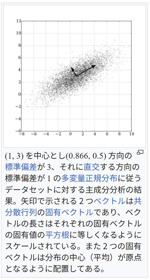
直感的な説明 主成分分析は与えられたデータを n 次元の楕円体にフィッティングするものであると考えることができる。このとき、それぞれの主成分は楕円体の軸に対応している。楕円体の軸が短いほどデータの分散は小さく、短い軸に対応する主成分を無視することで、データの分散と同程度に小さな情報の損失だけで、データをより少ない変数で表現することができる。
楕円体の軸を見つけるには、データの平均を座標軸の原点に合わせる必要がある。そのため、データの共分散行列を計算し、共分散行列に対する固有値と固有ベクトルを計算する。また、それぞれの固有ベクトルを直交化し、正規化する必要がある。固有ベクトルの組として互いに直交する単位ベクトルが得られたなら、それらに対応する軸を持つ楕円体によってデータをフィッティングすることができる。それぞれの軸に対する寄与率(proportion of the variance: 分散の比)は、その軸に対応する固有ベクトルに対する固有値を、すべての固有値の和で割ったものとして得ることができる。
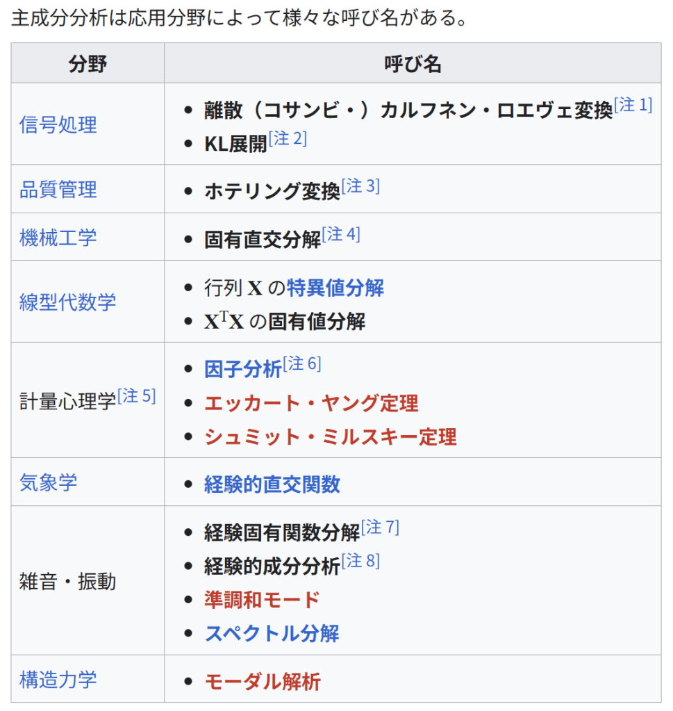
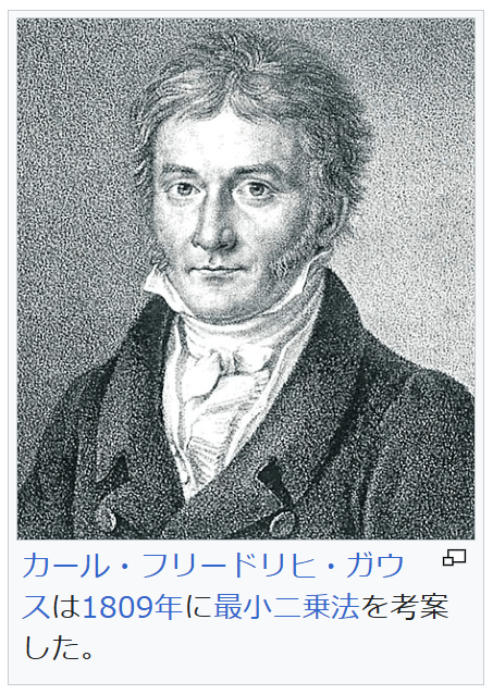
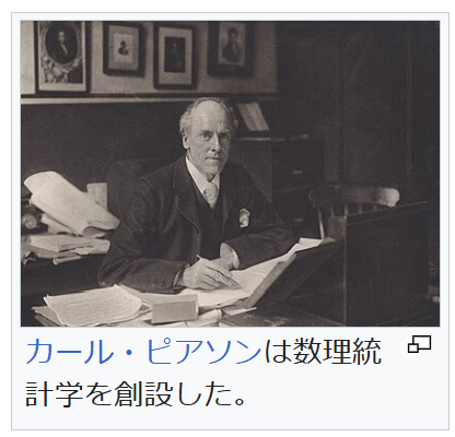
歴史と名称 主成分分析は1901年にカール・ピアソンによって導入された[4]。ピアソンは力学における主軸定理(英語版)からの類推によって主成分分析の方法を得た。主成分分析は、ピアソンとは独立に1930年代にハロルド・ホテリングよっても導入され、ホテリングによって主成分分析 (principal component analysis) と呼ばれるようになった[5][6]。(Jolliffe (2002, 1.2 A Brief History of Principal Component Analysis) 参照。)
以下では、データ行列 X として、各列の標本平均が 0 になるものを考える[注 9]。データ行列の各列 p はそれぞれデータが持つ特定の指標に対応し、データ行列の各行 n はそれぞれ異なる事例に対する指標の組を表す[注 10]。
主成分分析は p 次元ベクトル wk によってデータ行列 X の各行 xi を主成分得点のベクトル t(i) = (t1, …, tk)(i) に変換することであり、主成分得点tk(i) はデータ点 xi と負荷量ベクトル wk の内積によって与えられる。
t k ( i
)
x i ⋅ w k {\displaystyle {t_{k}}{(i)}=\mathbf {x} {i}\cdot \mathbf {w} _{k}} 負荷量ベクトル w は単位ベクトルであり、各主成分得点の分散を第一主成分から順に最大化するように選ばれる。負荷量ベクトルの個数(つまり主成分の数)k は、元の指標の数 p に等しいか、より小さい数が選ばれる (k ≤ p)。負荷量ベクトルの個数、つまり新しいデータ空間の次元を元の空間の次元より少なくとることで、次元削減をすることができる(#次元削減を参照)。主成分分析による次元削減は、データの分散に関する情報を残すように行われる。
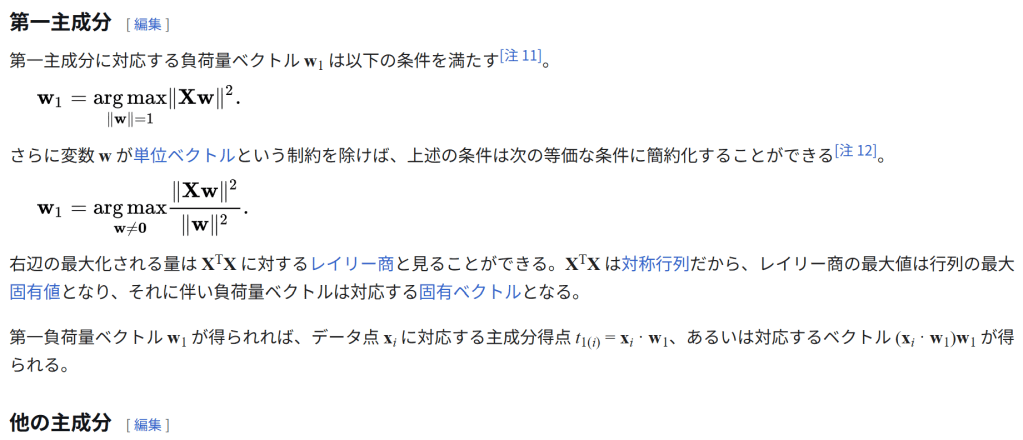
第一主成分 第一主成分に対応する負荷量ベクトル w1 は以下の条件を満たす[注 11]。
w
1
a r g m a x ‖ w
‖
1 ‖ X w ‖ 2 . {\displaystyle \mathbf {w} _{1}={\underset {\Vert \mathbf {w} \Vert =1}{\operatorname {arg\,max} }}\Vert \mathbf {Xw} \Vert ^{2}.} さらに変数 w が単位ベクトルという制約を除けば、上述の条件は次の等価な条件に簡約化することができる[注 12]。
w
1
a r g m a x w ≠ 0 ‖ X w ‖ 2 ‖ w ‖ 2 . {\displaystyle \mathbf {w} _{1}={\underset {\mathbf {w} \neq \mathbf {0} }{\operatorname {arg\,max} }}{\frac {\Vert \mathbf {Xw} \Vert ^{2}}{\Vert \mathbf {w} \Vert ^{2}}}.} 右辺の最大化される量は XTX に対するレイリー商と見ることができる。XTX は対称行列だから、レイリー商の最大値は行列の最大固有値となり、それに伴い負荷量ベクトルは対応する固有ベクトルとなる。
第一負荷量ベクトル w1 が得られれば、データ点 xi に対応する主成分得点 t1(i) = xi · w1、あるいは対応するベクトル (xi · w1)w1 が得られる。
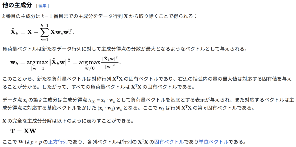
他の主成分 k 番目の主成分は k − 1 番目までの主成分をデータ行列 X から取り除くことで得られる:
X ^
k
X − ∑
s
1 k − 1 X w s w s T . {\displaystyle \mathbf {\hat {X}} {k}=\mathbf {X} -\sum {s=1}^{k-1}\mathbf {X} \mathbf {w} {s}\mathbf {w} {s}^{\rm {T}}.} 負荷量ベクトルは新たなデータ行列に対して主成分得点の分散が最大となるようなベクトルとして与えられる。
w
k
a r g m a x ‖ w
‖
1 ‖ X ^ k w ‖
2
a r g m a x w ≠ 0 ‖ X ^ k w ‖ 2 ‖ w ‖ 2 . {\displaystyle \mathbf {w} {k}={\underset {\Vert \mathbf {w} \Vert =1}{\operatorname {arg\,max} }}\Vert \mathbf {\hat {X}} {k}\mathbf {w} \Vert ^{2}={\underset {\mathbf {w} \neq \mathbf {0} }{\operatorname {arg\,max} }}{\tfrac {\Vert \mathbf {\hat {X}} _{k}\mathbf {w} \Vert ^{2}}{\Vert \mathbf {w} \Vert ^{2}}}.} このことから、新たな負荷量ベクトルは対称行列 XTX の固有ベクトルであり、右辺の括弧内の量の最大値は対応する固有値を与えることが分かる。したがって、すべての負荷量ベクトルは XTX の固有ベクトルである。
データ点 xi の第 k 主成分は主成分得点 tk(i) = xi · wk として負荷量ベクトルを基底とする表示が与えられ、また対応するベクトルは主成分得点に対応する基底ベクトルをかけた (xi · wk) wk となる。ここで wk は行列 XTX の第 k 固有ベクトルである。
X の完全な主成分分解は以下のように表わすことができる。
T
X W {\displaystyle \mathbf {T} =\mathbf {X} \mathbf {W} } ここで W は p × p の正方行列であり、各列ベクトルは行列の XTX の固有ベクトルであり単位ベクトルである。
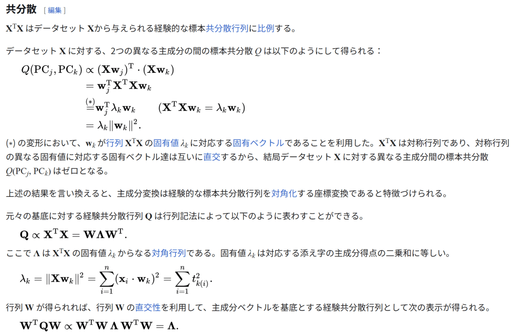
1 n t k ( i ) 2 . {\displaystyle \lambda {k}=|\mathbf {X} \mathbf {w} {k}|^{2}=\sum {i=1}^{n}(\mathbf {x} {i}\cdot \mathbf {w} {k})^{2}=\sum {i=1}^{n}t_{k(i)}^{2}.} 行列 W が得られれば、行列 W の直交性を利用して、主成分ベクトルを基底とする経験共分散行列として次の表示が得られる。
W T Q W ∝ W T W Λ W T
W
Λ . {\displaystyle \mathbf {W} ^{\mathrm {T} }\mathbf {Q} \mathbf {W} \propto \mathbf {W} ^{\mathrm {T} }\mathbf {W} \,\mathbf {\Lambda } \,\mathbf {W} ^{\mathrm {T} }\mathbf {W} =\mathbf {\Lambda } .} 次元削減 線型変換 T = XW はデータ点 xi を元の p 次元の空間から、与えられたデータセットに対して各成分が互いに無相関になるような p 次元の空間へ写すが、一部の主成分だけを残すような変換も考えることができる。第一主成分から順に、各主成分に関するデータの分散が単調減少するように負荷量ベクトルが得られるため、最初の L 個の負荷量ベクトルだけを残し、残りの説明能力の低い負荷量ベクトルを無視すると、次のような変換が得られる。
T
L
X W L {\displaystyle \mathbf {T} {L}=\mathbf {X} \mathbf {W} {L}} WL は p × L の行列であり、TL は n × L の行列である。上記の変換はデータ点 x ∈ Rp に対する変換として[注 13]、t = WTx (t ∈ RL) と書くこともできる。つまり、主成分分析は p 個の特徴量を持つデータ点 x を L 個の互いに無相関な特徴量を持つ主成分得点 t へ写す線型変換 W : Rp → RL を学習する手法であるといえる[10]。 データ行列を変換することで得られる主成分得点行列は、元のデータセットの分散を保存し、二乗再構成誤差 (reconstruction error) の総和、
‖ T W T − T L W L T ‖ 2 2 ( ‖ X − X L ‖ 2 2 ) {\displaystyle |\mathbf {T} \mathbf {W} ^{\mathrm {T} }-\mathbf {T} {L}\mathbf {W} {L}^{\mathrm {T} }|_{2}^{2}\qquad (|\mathbf {X} -\mathbf {X} {L}|{2}^{2})} を最小化するように与えられる。
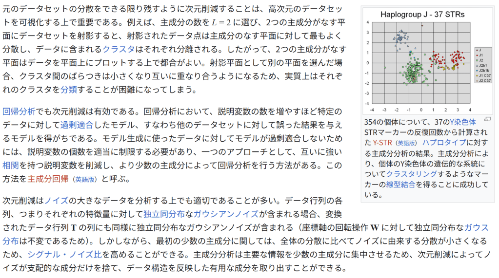
354の個体について、37のY染色体STRマーカーの反復回数から計算された Y-STR(英語版) ハプロタイプに対する主成分分析の結果。主成分分析により、個体のY染色体の遺伝的な系統についてクラスタリングするようなマーカーの線型結合を得ることに成功している。 元のデータセットの分散をできる限り残すように次元削減することは、高次元のデータセットを可視化する上で重要である。例えば、主成分の数を L = 2 に選び、2つの主成分がなす平面にデータセットを射影すると、射影されたデータ点は主成分のなす平面に対して最もよく分散し、データに含まれるクラスタはそれぞれ分離される。したがって、2つの主成分がなす平面はデータを平面上にプロットする上で都合がよい。射影平面として別の平面を選んだ場合、クラスタ間のばらつきは小さくなり互いに重なり合うようになるため、実質上はそれぞれのクラスタを分類することが困難になってしまう。
次元削減はノイズの大きなデータを分析する上でも適切であることが多い。データ行列の各列、つまりそれぞれの特徴量に対して独立同分布なガウシアンノイズが含まれる場合、変換されたデータ行列 T の列にも同様に独立同分布なガウシアンノイズが含まれる(座標軸の回転操作 W に対して独立同分布なガウス分布は不変であるため)。しかしながら、最初の少数の主成分に関しては、全体の分散に比べてノイズに由来する分散が小さくなるため、シグナル・ノイズ比を高めることができる。主成分分析は主要な情報を少数の主成分に集中させるため、次元削減によってノイズが支配的な成分だけを捨て、データ構造を反映した有用な成分を取り出すことができる。
特異値分解 主成分変換は行列の特異値分解とも結び付けられる。行列 X の特異値分解は以下の形式で与えられる。
X
U Σ W T . {\displaystyle \mathbf {X} =\mathbf {U} \mathbf {\Sigma } \mathbf {W} ^{\mathrm {T} }.} ここで、Σ は n × p の矩形対角行列であり、対角成分 σk が正の行列である。Σ の対角成分を行列 X の特異値という。U は n × n の正方行列であり、各列が互いに直交する n 次元の単位ベクトル[注 14]となる行列(つまり直交行列)である。各々の単位ベクトルは行列 X の左特異ベクトルと呼ばれる。同様に W は、各列が互いに直交する p 次元の単位ベクトルとなる p × p の正方行列である。こちらの単位ベクトルは行列 X の右特異ベクトルと呼ばれる。
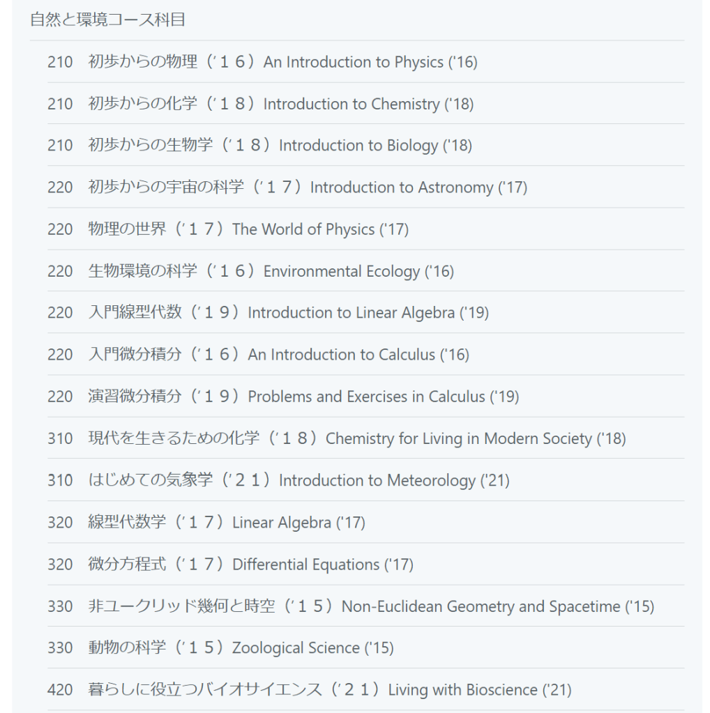
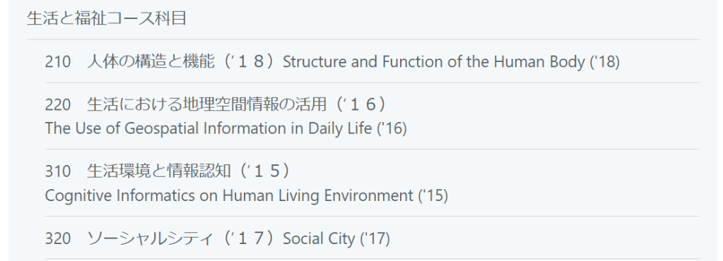
110 情報学へのとびら(’16)Introduction to Informatics (’16) 110 初歩からの数学(’18)Introduction to Mathematics (’18) 110 演習初歩からの数学(’20)Exercise in Introduction to Mathematics(’20) 110 自然科学はじめの一歩(’15) Introduction to Natural Sciences (’15) 110 運動と健康(’18)Exercise and Health Sciences (’18)
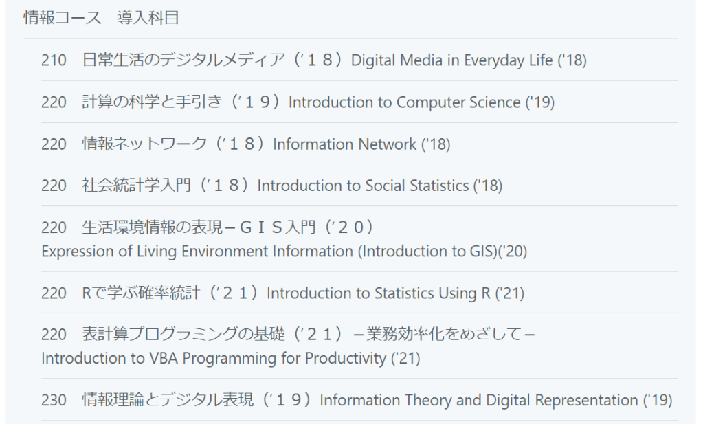
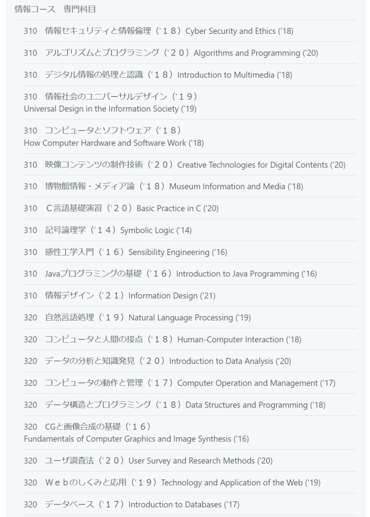
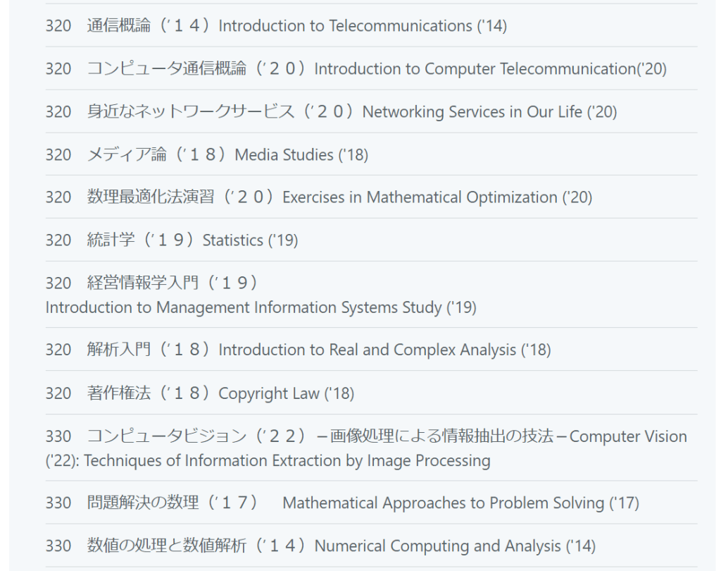
情報コース 導入科目
210 日常生活のデジタルメディア(’18)Digital Media in Everyday Life (’18) 220 計算の科学と手引き(’19)Introduction to Computer Science (’19)
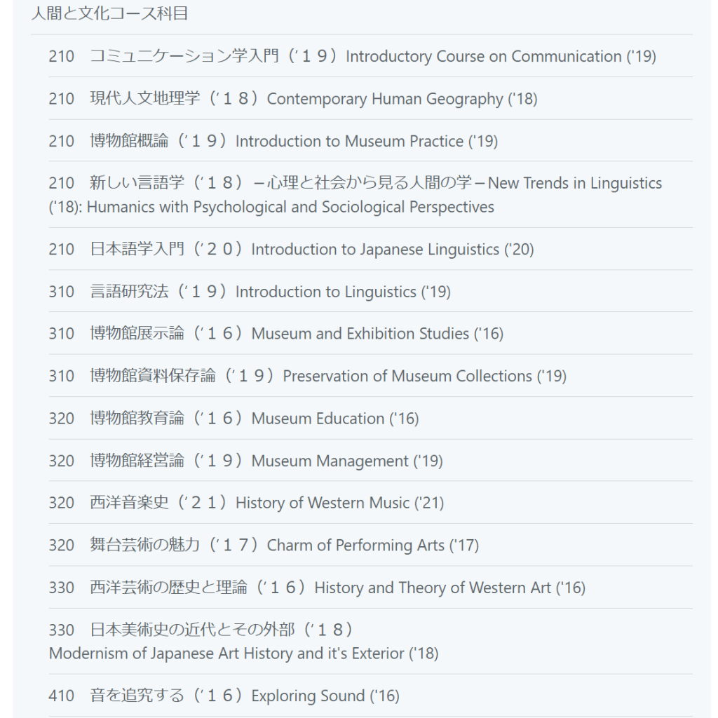
210 新しい言語学(’18)-心理と社会から見る人間の学- New Trends in Linguistics (’18): Humanics with Psychological and Sociological Perspectives 内容充実度:8 内容難易度:7 試験難易度:6 犬はゴーゴリと名付けよ
320 西洋音楽史(’21) History of Western Music (’21) 内容充実度:7 内容難易度:6 試験難易度:6
古代ギリシャから19世紀までの歴史的展開を追う構成です。我々が当たり前のように考えている「クラシック音楽」はどこに由来するのか?という問いが中心にあります。放送時間45分の制約で紹介される音源が限られているのでかなり理論面に寄っており、扱われた曲をちゃんと聞きたかったら自分で探さないと厳しいです(私はAmazon Music Unlimitedを契約して聞いてました。グレゴリオ聖歌とかマニアックなオペラとかも割とカバーしててAmazonすげー!となります。)。これを履修してから古楽に微ハマり中です。
320 舞台芸術の魅力(’17) Charm of Performing Arts (’17) 内容充実度:7 内容難易度:7 試験難易度:8
330 西洋芸術の歴史と理論(’16) History and Theory of Western Art (’16) 内容充実度:8 内容難易度:7 試験難易度:9
UIUXデザイナーという仕事柄、「芸術理論」というものに関心を持って履修しました。テレビ授業の本領発揮という感じでヨーロッパ各地の美術館や教会を巡りながら進んでいきます(お金あったんだなあ)。「芸術は芸術家の自己表現ではなく、世界表現である」というスタンスに立ち、時代時代の世界の捉え方を追いながら作品を解釈していきます。「ゴシック」「バロック」「ロココ」など、なんとなく聞いたことはあるけど何なのかよくわからなかった概念が整理されてすっきりした気持ちになれました。2021年から在宅試験向けに単位認定試験がチューニングされてありえないくらい難化してるので要注意です。 330 日本美術史の近代とその外部(’18) Modernism of Japanese Art History and it’s Exterior (’18) 内容充実度:8 内容難易度:7 試験難易度:?
グスタフ・フェヒナーは社会学的および心理学的現象で中央値 (Centralwerth) を用いた[22]。それ以前では天文学とその関連分野でしか使われていなかった。フランシス・ゴルトンは1881年に、初めて英語での用語として median を用いた。それより以前では、1869年に middle-most value が、1880年には medium が使用されていた[23]。
オックスフォード大学の学者であるフランシス・イシドロ・エッジワースは著書 “Metretike: or The Method of Measuring Probability and Utility” (1887) で、帰納的推論の基礎として確率を扱っており、彼の後の作品では「偶然の哲学」に焦点が当てられていた[26]。
彼の統計学に関する最初の論文 (1883) は誤差の法則(正規分布)を調べたものであった。
そして彼の “Methods of Statistics” (1885) では、t分布の初期のバージョン、エッジワース展開、エッジワース級数(英語版)、変数変換する方法、最尤推定の漸近理論が導入された。
社会情勢の統計調査は、チャールス・ブースの “Life and Labour of the People in London” (1889-1903)、シーボーム・ラウントリーの “Poverty, A Study of Town Life” (1901) に端を発したが、中でも革新的なのは、ボウリーの無作為抽出による手法である。彼の功績は “New Survey of London Life and Labour” で最高潮に達した[28]。
フィッシャーの論文 “On a distribution yielding the error functions of several well known statistics”(よく知られた統計集団の誤差関数を与える分布について、1924年)には、ピアソンのカイ二乗検定、正規分布と同じ構成での、ウィリアム・ゴセットのt分布、分散分析における、フィッシャーのz分布(英語版)(数十年後に、より一般化したF分布の形で用いられるようになる)の変数が示されている[38]。
この発想はさらに、ブルーノ・デ・フィネッティ(イタリア、Fondamenti Logici del Ragionamento Probabilistico, 1930)、フランク・ラムゼイ(ケンブリッジ、The Foundations of Mathematics, 1931)に取り入れられた[69]。
このアプローチは、統計的確率についての問題点を解決するために考案された。
これはラプラスの客観的なアプローチより前のことであった[68]。主観的なベイズ統計学の手法は、1950年代に Leonard Jimmie Savage によってさらに発展し普及した[要出典]。
客観的なベイズ推定はさらにハロルド・ジェフリーズ(ケンブリッジ大学)によって発展した。
彼の独創的な著書『確率論』(Theory of probability)が1939年に最初に登場し、ベイズ確率の再興に重要な役割を果たした[70][71]。
^ Ball, Philip (2004). Critical Mass. Farrar, Straus and Giroux. p. 53. ISBN 978-0-374-53041-9 ^ a b c 酒井弘憲「数式なしの統計のお話 第2回 統計のルーツを探る」『ファルマシア』第50巻第4号、2014年、334–335頁、doi:10.14894/faruawpsj.50.4_334。 ^ a b “意外に面白い!統計学を歴史から眺めてみよう!”. 数学・統計教室の和から株式会社 (2021年9月8日). 2022年11月29日閲覧。 ^ a b c 奥積雅彦. “公文書で初めて統計の用語が登場したのはいつか?” (PDF). 国立国会図書館支部総務省統計図書館. 2022年11月29日閲覧。 ^ Thucydides (1985). History of the Peloponnesian War. New York: Penguin Books, Ltd.. p. 204 ^ Giovanni Villani. Encyclopædia Britannica. Encyclopædia Britannica 2006 Ultimate Referece Suite DVD. Retrieved on 2008-03-04. ^ Brian, Éric; Jaisson, Marie (2007). “Physico-Theology and Mathematics (1710-1794)”. The Descent of Human Sex Ratio at Birth. Springer Science & Business Media. pp. 1-25. ISBN 978-1-4020-6036-6 ^ John Arbuthnot (1710). “An argument for Divine Providence, taken from the constant regularity observed in the births of both sexes”. Philosophical Transactions of the Royal Society of London 27 (325-336): 186-190. doi:10.1098/rstl.1710.0011. ^ a b Conover, W.J. (1999), “Chapter 3.4: The Sign Test”, Practical Nonparametric Statistics (Third ed.), Wiley, pp. 157-176, ISBN 978-0-471-16068-7 ^ Sprent, P. (1989), Applied Nonparametric Statistical Methods (Second ed.), Chapman & Hall, ISBN 978-0-412-44980-2 ^ Stephen Mack Stigler (1986). The History of Statistics: The Measurement of Uncertainty Before 1900. Harvard University Press. pp. 225-226. ISBN 978-0-67440341-3 ^ Bellhouse, P. (2001), “John Arbuthnot”, in Statisticians of the Centuries by C.C. Heyde and E. Seneta, Springer, pp. 39-42, ISBN 978-0-387-95329-8 ^ Hald, Anders (1998), “Chapter 4. Chance or Design: Tests of Significance”, A History of Mathematical Statistics from 1750 to 1930, Wiley, p. 65 ^ Abraham de Moivre (1738) The doctrine of chances. Woodfall ^ P=S Laplace (1774). “Mémoire sur la probabilité des causes par les évènements”. Mémoires de l’Académie Royale des Sciences Présentés par Divers Savants 6: 621-656. ^ Wilson, Edwin Bidwell (1923) “First and second laws of error”, Journal of the American Statistical Association, 18 (143), 841-851 JSTOR 2965467 ^ Havil J (2003) Gamma: Exploring Euler’s Constant. Princeton, NJ: Princeton University Press, p.157 ^ Charles Sanders Peirce (1873) Theory of errors of observations. Report of the Superintendent US Coast Survey, Washington, Government Printing Office. Appendix no. 21: 200-224 ^ P. S. Laplace (1781). “MEMOIRE SUR LES PROBABILITÉS”. Oeuvres completes 9: 227-332. 英語訳PDF ^ ウィキソースのロゴ フランス語版ウィキソースに本記事に関連した原文があります:Page:Laplace_-_Œuvres_complètes,_Gauthier-Villars,_1878,_tome_9.djvu/395 ^ William Gemmell Cochran (1978) “Laplace’s ratio estimators”. pp.3-10. In David H.A., (ed). Contributions to Survey Sampling and Applied Statistics: papers in honor of H. O. Hartley. Academic Press, New York ISBN 978-1483237930 ^ John Maynard Keynes (1921) A treatise on probability. Pt II Ch XVII §5 (p 201) ^ Francis Galton (1881) Report of the Anthropometric Committee pp.245-260. Report of the 51st Meeting of the British Association for the Advancement of Science ^ Stigler (1986, Chapter 5: Quetelet’s Two Attempts) ^ Helen Mary Walker (1975). Studies in the history of statistical method. Arno Press. ISBN 9780405066283 ^ (Stigler 1986, Chapter 9: The Next Generation: Edgeworth) ^ Bellhouse DR (1988) A brief history of random sampling methods. Handbook of statistics. Vol 6 pp.1-14 Elsevier ^ Bowley, AL (1906). “Address to the Economic Science and Statistics Section of the British Association for the Advancement of Science”. J R Stat Soc 69: 548-557. doi:10.2307/2339344. JSTOR 2339344. ^ Francis Galton (1877). “Typical laws of heredity”. Nature 15 (388): 492-553. doi:10.1038/015492a0. ^ Francis Galton (1907). “One Vote, One Value”. Nature 75 (1948): 414. doi:10.1038/075414a0. ^ Stigler (1986, Chapter 10: Pearson and Yule) ^ Varberg, Dale E. (1963). “The development of modern statistics”. The Mathematics Teacher 56 (4): 252-257. JSTOR 27956805. ^ Stephen Mack Stigler (1989). “Francis Galton’s Account of the Invention of Correlation”. Statistical Science 4 (2): 73-79. doi:10.1214/ss/1177012580. ^ a b c Karl Pearson (1900). “On the Criterion that a given System of Deviations from the Probable in the Case of a Correlated System of Variables is such that it can be reasonably supposed to have arisen from Random Sampling”. Philosophical Magazine. Series 5 50 (302): 157-175. doi:10.1080/14786440009463897. ^ Karl Pearson (1901). “On Lines and Planes of Closest Fit to Systems of Points is Space”. Philosophical Magazine. Series 6 2 (11): 559-572. doi:10.1080/14786440109462720. ^ I.T. Jolliffe (2002) Principal Component Analysis, 2nd ed. New York: Springer-Verlag. ^ Box, R.A. Fisher, pp.93-166 ^ Agresti, Alan; David B. Hichcock (2005). “Bayesian Inference for Categorical Data Analysis”. Statistical Methods & Applications 14 (3): 298. doi:10.1007/s10260-005-0121-y. ^ R.A. Fisher (1925) Statistical methods for research workers, Edinburgh: Oliver & Boyd ^ Jerzy Neyman (1934) On the two different aspects of the representative method: The method of stratified sampling and the method of purposive selection. Journal of the Royal Statistical Society 97 (4) 557-625 JSTOR 2342192 ^ Dunn, Peter (1997-01). “James Lind (1716-94) of Edinburgh and the treatment of scurvy”. Archives of Disease in Childhood: Fetal and Neonatal Edition 76 (1): 64-65. doi:10.1136/fn.76.1.F64. PMC 1720613. PMID 9059193. ^ a b Klaus Hinkelmann (2012). Design and Analysis of Experiments, Special Designs and Applications. John Wiley & Sons. p. xvii. ISBN 9780470530689 ^ a b Charles Sanders Peirce, Joseph Jastrow (1885). “On Small Differences in Sensation”. Memoirs of the National Academy of Sciences 3: 73-83. ^ a b Ian Hacking (1988-09). “Telepathy: Origins of Randomization in Experimental Design”. Isis 79 (A Special Issue on Artifact and Experiment, number 3): 427-451. doi:10.1086/354775. JSTOR 234674. MR1013489. ^ a b Stephen Mack Stigler (1992-11). “A Historical View of Statistical Concepts in Psychology and Educational Research”. American Journal of Education 101 (1): 60-70. doi:10.1086/444032. ^ a b Trudy Dehue (1997-12). “Deception, Efficiency, and Random Groups: Psychology and the Gradual Origination of the Random Group Design”. Isis 88 (4): 653-673. doi:10.1086/383850. PMID 9519574. ^ C.S. Peirce (1876). “Note on the Theory of the Economy of Research”. Coast Survey Report: 197-201., actually published 1879, NOAA PDF Eprint. Reprinted in Collected Papers 7, paragraphs 139-157, also in Writings 4, pp.72-78, and in Charles Sanders Peirce (1967年7-8月). “Note on the Theory of the Economy of Research”. Operations Research 15 (4): 643-648. doi:10.1287/opre.15.4.643. JSTOR 168276. ^ Smith, Kirstine (1918). “On the Standard Deviations of Adjusted and Interpolated Values of an Observed Polynomial Function and its Constants and the Guidance they give Towards a Proper Choice of the Distribution of Observations”. Biometrika 12 (1/2): 1-85. doi:10.2307/2331929. JSTOR 2331929. ^ Abraham Wald (1945) “Sequential Tests of Statistical Hypotheses”, Annals of Mathematical Statistics, 16 (2), 117-186. ^ Johnson, N.L. (1961). “Sequential analysis: a survey.” Journal of the Royal Statistical Society, Series A. Vol. 124 (3), 372-411. (pages 375-376) ^ Herman Chernoff (1972) Sequential Analysis and Optimal Design, SIAM Monograph. ISBN 978-0898710069 ^ Zacks, S. (1996) “Adaptive Designs for Parametric Models”. In: Ghosh, S. and Rao, C. R., (Eds) (1996). “Design and Analysis of Experiments,” Handbook of Statistics, Volume 13. North-Holland. ISBN 0-444-82061-2. (pp.151-180) ^ Robbins, H. (1952). “Some Aspects of the Sequential Design of Experiments”. Bulletin of the American Mathematical Society 58 (5): 527-535. doi:10.1090/S0002-9904-1952-09620-8. ^ Hald, Anders (1998) A History of Mathematical Statistics. New York: Wiley. [要ページ番号] ^ Box, Joan Fisher (1978) R. A. Fisher: The Life of a Scientist, Wiley. ISBN 0-471-09300-9 (pp.93-166) ^ Edwards, A.W.F. (2005). “R. A. Fisher, Statistical Methods for Research Workers, 1925”. In Grattan-Guinness, Ivor. Landmark writings in Western mathematics 1640-1940. Amsterdam Boston: Elsevier. ISBN 9780444508713 ^ Stanley, J. C. (1966). “The Influence of Fisher’s “The Design of Experiments” on Educational Research Thirty Years Later”. American Educational Research Journal 3 (3): 223-229. doi:10.3102/00028312003003223. ^ Box, JF (1980-02). “R. A. Fisher and the Design of Experiments, 1922-1926”. The American Statistician 34 (1): 1-7. doi:10.2307/2682986. JSTOR 2682986. ^ Frank Yates (1964-06). “Sir Ronald Fisher and the Design of Experiments”. Biometrics 20 (2): 307-321. doi:10.2307/2528399. JSTOR 2528399. ^ Stanley, Julian C. (1966). “The Influence of Fisher’s “The Design of Experiments” on Educational Research Thirty Years Later”. American Educational Research Journal 3 (3): 223-229. doi:10.3102/00028312003003223. JSTOR 1161806. ^ a b c Stigler (1986, Chapter 3: Inverse Probability) ^ Hald (1998)[要ページ番号] ^ Lucien Le Cam (1986) Asymptotic Methods in Statistical Decision Theory: pp.336, 618-621(von Mises と Bernstein). ^ a b c Stephen. E. Fienberg, (2006) When did Bayesian Inference become “Bayesian”? Archived 2014-09-10 at the Wayback Machine. Bayesian Analysis, 1 (1), 1-40. See page 5. ^ a b Aldrich, A (2008). “R. A. Fisher on Bayes and Bayes’ Theorem”. Bayesian Analysis 3 (1): 161-170. doi:10.1214/08-ba306. ^ Jerzy Neyman (1977). “Frequentist probability and frequentist statistics”. Synthese 36 (1): 97-131. doi:10.1007/BF00485695. ^ Jeff Miller, “Earliest Known Uses of Some of the Words of Mathematics (B)” “The term Bayesian entered circulation around 1950. R. A. Fisher used it in the notes he wrote to accompany the papers in his Contributions to Mathematical Statistics (1950). Fisher thought Bayes’s argument was all but extinct for the only recent work to take it seriously was Harold Jeffreys’s Theory of Probability (1939). In 1951 L. J. Savage, reviewing Wald’s Statistical Decisions Functions, referred to “modern, or unBayesian, statistical theory” (“The Theory of Statistical Decision,” Journal of the American Statistical Association, 46, p.58.). Soon after, however, Savage changed from being an unBayesian to being a Bayesian.” ^ a b c José-Miguel Bernardo (2005). “Reference analysis”. Bayesian Thinking – Modeling and Computation. Handbook of Statistics. 25. pp. 17-90. doi:10.1016/S0169-7161(05)25002-2. ISBN 9780444515391 ^ Donald A. Gillies (2000), Philosophical Theories of Probability. Routledge. ISBN 0-415-18276-X pp.50-1 ^ E.T. Jaynes Probability Theory: The Logic of Science Cambridge University Press, (2003). ISBN 0-521-59271-2 ^ O’Connor, John J.; Robertson, Edmund F., “統計学の歴史”, MacTutor History of Mathematics archive, University of St Andrews. ^ J.M. Bernardo, A.F.M. Smith (1994). “Bayesian Theory”. Chichester: Wiley. ^ Wolpert, RL (2004). “A conversation with James O. Berger”. Statistical Science 9: 205-218. doi:10.1214/088342304000000053. MR2082155. ^ Bernardo, J.M. (2006). “A Bayesian Mathematical Statistics Primer” (PDF). Proceedings of the Seventh International Conference on Teaching Statistics [CDROM]. Salvador (Bahia), Brazil: International Association for Statistical Education. ^ C.M. Bishop (2007) Pattern Recognition and Machine Learning. Springer ISBN 978-0387310732 ^ 統計学の歴史〜古代ローマから現代まで〜 | AVILEN AI Trend 2020年4月14日、2022年6月26日閲覧。 参考文献 Freedman, D. (1999). “From association to causation: Some remarks on the history of statistics”. Statistical Science 14 (3): 243-258. doi:10.1214/ss/1009212409. (Revised version, 2002) Anders Hald (2003). A History of Probability and Statistics and Their Applications before 1750. Hoboken, NJ: Wiley. ISBN 978-0-471-47129-5 Anders Hald (1998). A History of Mathematical Statistics from 1750 to 1930. New York: Wiley. ISBN 978-0-471-17912-2 Kotz, S., Johnson, N.L. (1992,1992,1997). Breakthroughs in Statistics, Vols I, II, III. Springer ISBN 0-387-94037-5, 0-387-94039-1, 0-387-94989-5 エゴン・ピアソン (1978). The History of Statistics in the 17th and 18th Centuries against the changing background of intellectual, scientific and religious thought(カール・ピアソンによる、ユニヴァーシティ・カレッジ・ロンドンの 1921-1933 の academic session での講義). New York: MacMillan Publishing Co., Inc.. p. 744. ISBN 978-0-02-850120-8 David Salsburg (2001). The Lady Tasting Tea: How Statistics Revolutionized Science in the Twentieth Century. ISBN 0-7167-4106-7 スティーブン・スティグラー (1986). The History of Statistics: The Measurement of Uncertainty before 1900. Belknap Press/Harvard University Press. ISBN 978-0-674-40341-3 スティーブン・スティグラー (1999) Statistics on the Table: The History of Statistical Concepts and Methods. ハーバード大学出版局。ISBN 0-674-83601-4 David, H.A. (1995). “First (?) Occurrence of Common Terms in Mathematical Statistics”. The American Statistician 49 (2): 121-133. doi:10.2307/2684625. JSTOR 2684625. 外部リンク
ウィキメディア・コモンズには、統計学の歴史に関連するカテゴリがあります。 JEHPS: Recent publications in the history of probability and statistics Electronic Journ@l for History of Probability and Statistics/Journ@l Electronique d’Histoire des Probabilités et de la Statistique Figures from the History of Probability and Statistics – サウサンプトン大学(イギリスの旗 イギリス) Materials for the History of Statistics – ヨーク大学(イギリスの旗 イギリス) Probability and Statistics on the Earliest Uses Pages – サウサンプトン大学(イギリスの旗 イギリス) Earliest Uses of Symbols in Probability and Statistics – Earliest Uses of Various Mathematical Symbols 表話編歴 統計学 カテゴリ: 科学史確率と統計分野別の科学史 最終更新 2024年10月19日 (土) 16:11 (日時は個人設定で未設定ならばUTC)。 テキストはクリエイティブ・コモンズ 表示-継承ライセンスのもとで利用できます。追加の条件が適用される場合があります。詳細については利用規約を参照してください。』